Linear Regression for Prediction

Lucy D’Agostino McGowan

`Application Exercise`

1. Create a new project from this template in RStudio Pro:

https://github.com/sta-363-f25/04-ex.git

2. Load the packages and data by running the top chunk of R code

Let’s look at an example

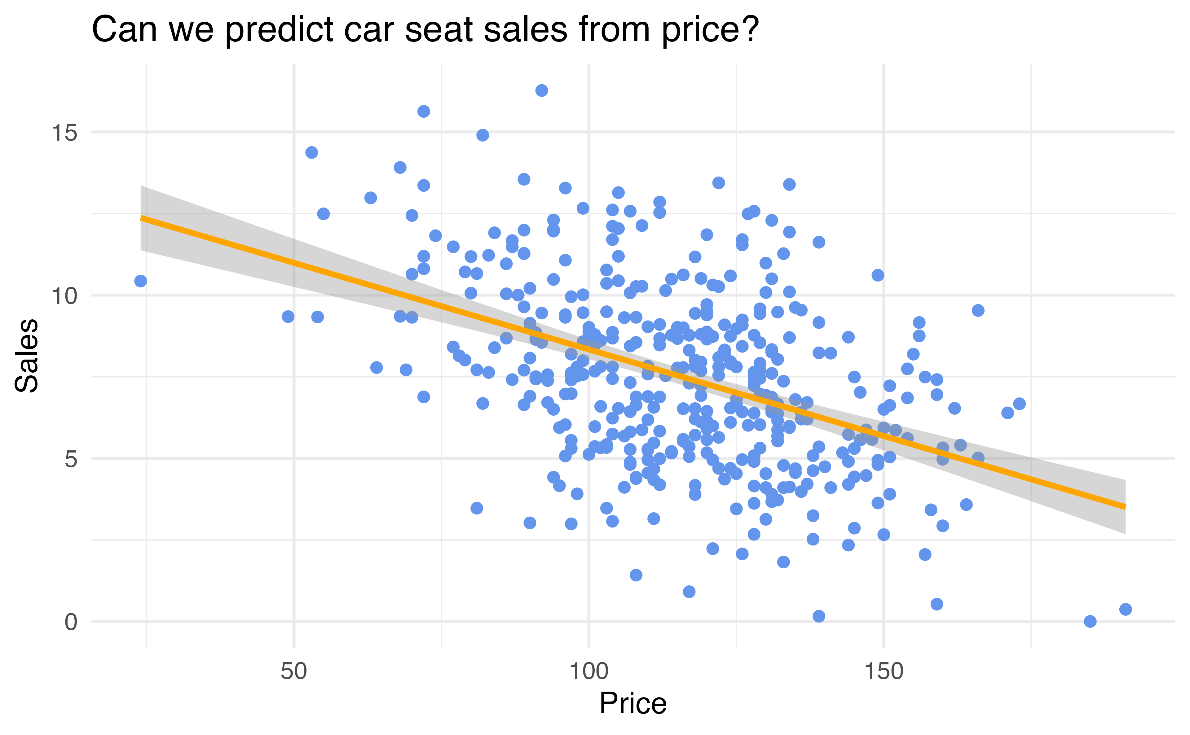
Let’s look at car seat sales data from 400 different stores. We want to predict Sales from Price

Building a Prediction Model

# Fit the model
carseat_fit <- linear_reg() |>
  set_engine("lm") |>
  fit(Sales ~ Price, data = Carseats)

# Look at the coefficients
carseat_fit |> tidy()

# A tibble: 2 × 5
  term        estimate std.error statistic  p.value
  <chr>          <dbl>     <dbl>     <dbl>    <dbl>
1 (Intercept)  13.6      0.633       21.6  7.46e-69
2 Price        -0.0531   0.00535     -9.91 7.62e-21

Making Predictions

If I sell my car seats for $200, how many do you predict that I will sell?

# Manual calculation
# Sales = 13.6 - 0.053 x 200
13.6 - 0.053 * 200

[1] 3

Making Predictions with `predict()`

# Create new data
new_carseat <- tibble(Price = 200)

# Make prediction
carseat_fit |> 
  predict(new_data = new_carseat)

# A tibble: 1 × 1
  .pred
  <dbl>
1  3.03

Multiple Predictions at Once

# Predict for several prices
new_carseats <- tibble(Price = c(100, 150, 200, 500, 1000))

predictions <- carseat_fit |> 
  predict(new_data = new_carseats)

# Combine with original data
bind_cols(new_carseats, predictions)

# A tibble: 5 × 2
  Price  .pred
  <dbl>  <dbl>
1   100   8.33
2   150   5.68
3   200   3.03
4   500 -12.9 
5  1000 -39.4

`Application Exercise`

Run this code to create a simulated dataset:

library(MASS)
set.seed(1)

# Generate 5 correlated X variables
Sigma <- matrix(0.25, 5, 5)
diag(Sigma) <- 1
X_mat <- mvrnorm(n = 20, mu = rep(0, 5), Sigma = Sigma)

# Generate Y with known relationship + noise
Y <- 2 + 3*X_mat[,1] - 1.5*X_mat[,2] + 0.5*X_mat[,3] + 
    0*X_mat[,4] + 0*X_mat[,5] + rnorm(20, 0, 0.5)

# Create data frame
sim_data <- tibble(
  X1 = X_mat[,1], X2 = X_mat[,2], X3 = X_mat[,3], 
  X4 = X_mat[,4], X5 = X_mat[,5], Y = Y
)

Fit a linear model predicting Y from all 5 X variables using linear_reg()
Make predictions for new observations where all X variables = 0, 1, and 2
Which set of X values gives the highest predicted Y?

05:00

Solution 1

# 2. Fit the model
sim_fit <- linear_reg() |>
  set_engine("lm") |>
  fit(Y ~ X1 + X2 + X3 + X4 + X5, data = sim_data)

sim_fit |> tidy()

# 3. Make predictions
new_obs <- tibble(
  X1 = c(0, 1, 2), X2 = c(0, 1, 2), X3 = c(0, 1, 2),
  X4 = c(0, 1, 2), X5 = c(0, 1, 2)
)

predictions <- sim_fit |>
  predict(new_data = new_obs) |>
  bind_cols(new_obs)

predictions

How Good Are Our Predictions?

Let’s look at prediction accuracy on our training data:

# Get predictions for all training data
training_results <- carseat_fit |>
  predict(new_data = Carseats) |>
  bind_cols(Carseats)

# Look at first few rows
training_results |> 
  select(Sales, .pred, Price) |> 
  head()

# A tibble: 6 × 3
  Sales .pred Price
  <dbl> <dbl> <dbl>
1  9.5   7.27   120
2 11.2   9.24    83
3 10.1   9.40    80
4  7.4   8.49    97
5  4.15  6.85   128
6 10.8   9.82    72

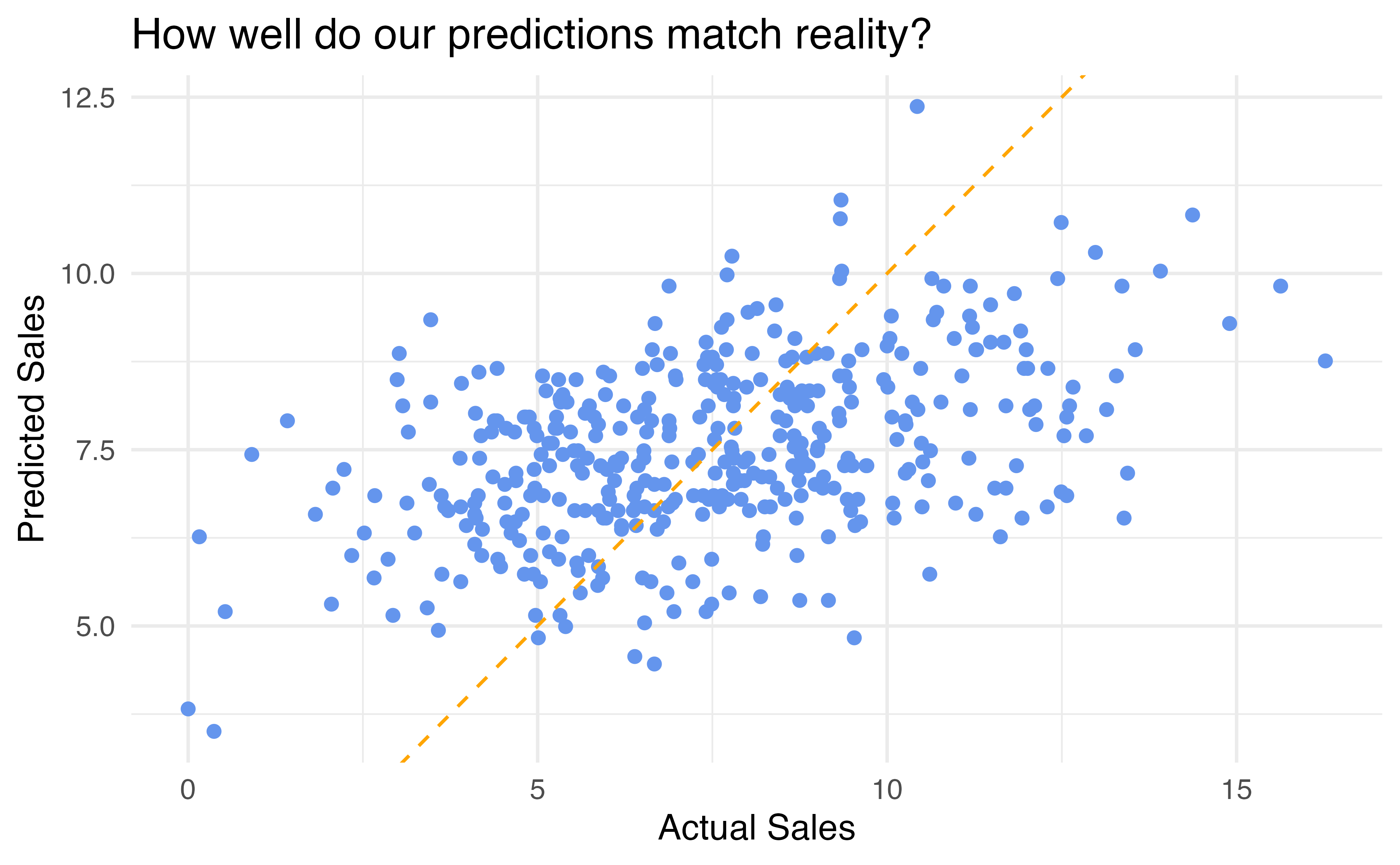
Visualizing Predictions vs Reality

ggplot(training_results, aes(x = Sales, y = .pred)) +
  geom_point(color = "cornflower blue") +
  geom_abline(slope = 1, intercept = 0, color = "orange", linetype = "dashed") +
  labs(x = "Actual Sales", y = "Predicted Sales",
       title = "How well do our predictions match reality?") +
  theme_minimal()

Measuring Prediction Accuracy: RMSE

Root Mean Squared Error (RMSE): Average prediction error

training_results |> 
  rmse(truth = Sales, estimate = .pred)

# A tibble: 1 × 3
  .metric .estimator .estimate
  <chr>   <chr>          <dbl>
1 rmse    standard        2.53

What does an RMSE of 2.5 mean in the context of carseat sales?

Measuring Prediction Accuracy: R²

R-squared: Proportion of variance explained by the model

training_results |> 
  rsq(truth = Sales, estimate = .pred)

# A tibble: 1 × 3
  .metric .estimator .estimate
  <chr>   <chr>          <dbl>
1 rsq     standard       0.198

How do we interpret R² = 0.2?

The Problem with Training Accuracy

Is training R² = 0.2 a good estimate of how well our model will predict new sales?

Problem: We’re testing the model on the same data we used to train it!

Cross-Validation for Better Estimates

# Create cross-validation folds
set.seed(1)
carseat_folds <- vfold_cv(Carseats, v = 5)

# Fit model on each fold and test on held-out data
cv_results <- linear_reg() |>
  fit_resamples(
    Sales ~ Price,
    resamples = carseat_folds
  )

# Get test performance metrics
collect_metrics(cv_results)

# A tibble: 2 × 6
  .metric .estimator  mean     n std_err .config             
  <chr>   <chr>      <dbl> <int>   <dbl> <chr>               
1 rmse    standard   2.54      5  0.0717 Preprocessor1_Model1
2 rsq     standard   0.202     5  0.0308 Preprocessor1_Model1

Training vs Test Performance

Metric	Training	Cross-Validation
RMSE	2.5	2.5
R-squared	0.2	0.2

What do you notice about training vs cross-validation performance?

`Application Exercise`

Using your simulated data, create the design matrix X (including intercept column)
Calculate the coefficients manually using: solve(crossprod(X)) %*% t(X) %*% y
Compare these coefficients to what you got from linear_reg() |> tidy()
Try changing the noise standard deviation from 0.5 to 2.0 - how do the predictions change for X₁=1, X₂=0, X₃=0, X₄=0, X₅=0?

06:00

Solution 2

# 1. Create design matrix
X_design <- cbind(1, X_mat)  # Add intercept column
y_vec <- sim_data$Y

# 2. Calculate coefficients manually
manual_coefs <- solve(crossprod(X_design)) %*% t(X_design) %*% y_vec
manual_coefs

# 3. Compare to tidymodels
sim_fit |> tidy()  # Should be very similar!

# 4. Change noise level
Y_noisy <- 2 + 3*X_mat[,1] - 1.5*X_mat[,2] + 0.5*X_mat[,3] + 
           0*X_mat[,4] + 0*X_mat[,5] + rnorm(20, 0, 2.0)

sim_data_noisy <- tibble(
  X1 = X_mat[,1], X2 = X_mat[,2], X3 = X_mat[,3], 
  X4 = X_mat[,4], X5 = X_mat[,5], Y = Y_noisy
)

noisy_fit <- linear_reg() |>
  set_engine("lm") |>
  fit(Y ~ X1 + X2 + X3 + X4 + X5, data = sim_data_noisy)

test_point <- tibble(X1 = 1, X2 = 0, X3 = 0, X4 = 0, X5 = 0)
sim_fit |> predict(test_point, type = "pred_int")    # Low noise
noisy_fit |> predict(test_point, type = "pred_int")  # High noise - wider intervals!

More Complex Predictions

multi_fit <- linear_reg() |>
  fit(Sales ~ Price + Income + Advertising +
        Population + ShelveLoc + Age +
        Education + Urban + US,
      data = Carseats)

# Cross-validate this more complex model
multi_cv <- linear_reg() |>
  fit_resamples(
    Sales ~ Price + Income + Advertising +
        Population + ShelveLoc + Age +
        Education + Urban + US,
    resamples = carseat_folds
  )

collect_metrics(multi_cv)

# A tibble: 2 × 6
  .metric .estimator  mean     n std_err .config             
  <chr>   <chr>      <dbl> <int>   <dbl> <chr>               
1 rmse    standard   1.57      5  0.0411 Preprocessor1_Model1
2 rsq     standard   0.691     5  0.0190 Preprocessor1_Model1

Comparing Model Complexity

Model	Predictors	Training R²	CV R²	Training RMSE	CV RMSE
Simple	Price only	0.20	0.20	2.5	2.5
Complex	9 predictors	0.71	0.69	1.5	1.6

Which model would you choose for prediction? Why?

Prediction Uncertainty

Our predictions aren’t perfect - how can we quantify uncertainty?

new_prices <- tibble(Price = c(100, 150, 200))

carseat_fit |>
  predict(new_data = new_prices, type = "pred_int") |>
  bind_cols(new_prices)

# A tibble: 3 × 3
  .pred_lower .pred_upper Price
        <dbl>       <dbl> <dbl>
1       3.35        13.3    100
2       0.683       10.7    150
3      -2.04         8.09   200

If we price our car seats at $150, we predict to sell 5,683 units, but the actual sales will likely be between 683 and 10,683 units.

`Application Exercise`

Create three simulations with different noise levels: sd = 0.1, 1.0, 3.0
For each noise level, make predictions for X₁=1, X₂=0, X₃=0, X₄=0, X₅=0
Plot the predicted values with prediction intervals
How do prediction intervals change with noise level?

06:00

Solution 3

set.seed(3)
noise_levels <- c(0.1, 1.0, 3.0)
results <- tibble()

for(i in seq_along(noise_levels)) {
  # Generate data with different noise
  Y_noise <- 2 + 3*X_mat[,1] - 1.5*X_mat[,2] + 0.5*X_mat[,3] + 
             0*X_mat[,4] + 0*X_mat[,5] + rnorm(20, 0, noise_levels[i])
  
  sim_data_temp <- tibble(
    X1 = X_mat[,1], X2 = X_mat[,2], X3 = X_mat[,3], 
    X4 = X_mat[,4], X5 = X_mat[,5], Y = Y_noise
  )
  
  # Fit model and predict
  temp_fit <- linear_reg() |>
    set_engine("lm") |>
    fit(Y ~ X1 + X2 + X3 + X4 + X5, data = sim_data_temp)
  
  pred <- temp_fit |>
    predict(sim_data_temp, type = "pred_int") |>
    bind_cols(sim_data_temp) |>
    mutate(noise_level = noise_levels[i])
  
  results <- bind_rows(results, pred)
}

# Plot results
ggplot(results, aes(x = Y)) +
  geom_errorbar(aes(ymin = .pred_lower, ymax = .pred_upper), width = 0.1) +
  labs(x = "Observed Y", y = "Predicted Y") +
  theme_minimal() + 
  facet_wrap(~noise_level)

Key Prediction Concepts

Goal: Build models that predict well on new, unseen data
Training accuracy is optimistic - always use cross-validation
RMSE measures average prediction error (in original units)
R² measures proportion of variance explained (0-1 scale)
Prediction intervals quantify uncertainty in individual predictions
Irreducible error affects prediction uncertainty
More complex models may predict better, but watch for overfitting

Understanding Prediction Uncertainty

Prediction intervals tell us how uncertain we are about individual predictions
Wider intervals = more uncertainty
Uncertainty comes from:
Estimation uncertainty: We don’t know the true coefficients perfectly
Irreduciable error: There’s natural noise in the data

Linear Regression for Prediction

Application Exercise

Let’s look at an example

Building a Prediction Model

Making Predictions

Making Predictions with predict()

Multiple Predictions at Once

Application Exercise

Solution 1

How Good Are Our Predictions?

Visualizing Predictions vs Reality

Measuring Prediction Accuracy: RMSE

Measuring Prediction Accuracy: R²

The Problem with Training Accuracy

Cross-Validation for Better Estimates

Training vs Test Performance

Application Exercise

Solution 2

More Complex Predictions

Comparing Model Complexity

Prediction Uncertainty

Application Exercise

Solution 3

Key Prediction Concepts

Understanding Prediction Uncertainty

`Application Exercise`

Making Predictions with `predict()`

`Application Exercise`

`Application Exercise`

`Application Exercise`