tidymodels

Application Exercise

tidymodels

lm_spec <- 
  linear_reg() |> # Pick linear regression
  set_engine(engine = "lm") # set engine
lm_spec

Linear Regression Model Specification (regression)

Computational engine: lm 

lm_fit <- fit(lm_spec,
              mpg ~ horsepower,
              data = Auto)

Validation set approach

Auto_split <- initial_split(Auto, prop = 0.5)
Auto_split

<Training/Testing/Total>
<196/196/392>

Extract the training and testing data

training(Auto_split)
testing(Auto_split)

A faster way!

• You can use last_fit() and specify the split
• This will automatically train the data on the train data from the split
• Instead of specifying which metric to calculate (with rmse as before) you can just use collect_metrics() and it will automatically calculate the metrics on the test data from the split

A faster way!

set.seed(100)

Auto_split <- initial_split(Auto, prop = 0.5)
lm_fit <- last_fit(lm_spec,
                   mpg ~ horsepower,
                   split = Auto_split) 

lm_fit |>
  collect_metrics() 

# A tibble: 2 × 4
  .metric .estimator .estimate .config             
  <chr>   <chr>          <dbl> <chr>               
1 rmse    standard       4.96  Preprocessor1_Model1
2 rsq     standard       0.613 Preprocessor1_Model1

What about cross validation?

Auto_cv <- vfold_cv(Auto, v = 5)
Auto_cv

#  5-fold cross-validation 
# A tibble: 5 × 2
  splits           id   
  <list>           <chr>
1 <split [313/79]> Fold1
2 <split [313/79]> Fold2
3 <split [314/78]> Fold3
4 <split [314/78]> Fold4
5 <split [314/78]> Fold5

What if we wanted to do some preprocessing

• For the shrinkage methods we discussed it was important to scale the variables

What does this mean?

What would happen if we scale before doing cross-validation? Will we get different answers?

What if we wanted to do some preprocessing

Auto_scaled <- Auto |>
  mutate(horsepower = scale(horsepower))

sd(Auto_scaled$horsepower)

[1] 1

Auto_cv_scaled <- vfold_cv(Auto_scaled, v = 5)

map_dbl(Auto_cv_scaled$splits,
        function(x) {
          dat <- as.data.frame(x)$horsepower
          sd(dat)
        })

[1] 1.0244697 1.0261352 0.9662367 0.9832638 0.9969558

What if we wanted to do some preprocessing

• recipe()!
• Using the recipe() function along with step_*() functions, we can specify preprocessing steps and R will automagically apply them to each fold appropriately.

rec <- recipe(mpg ~ horsepower, data = Auto) |>
  step_scale(horsepower) 

• You can find all of the potential preprocessing steps here: https://tidymodels.github.io/recipes/reference/index.html

Where do we plug in this recipe?

• The recipe gets plugged into the fit_resamples() function

Auto_cv <- vfold_cv(Auto, v = 5)

rec <- recipe(mpg ~ horsepower, data = Auto) |>
  step_scale(horsepower)

results <- fit_resamples(lm_spec,
                         preprocessor = rec,
                         resamples = Auto_cv)

results |>
  collect_metrics()

# A tibble: 2 × 6
  .metric .estimator  mean     n std_err .config             
  <chr>   <chr>      <dbl> <int>   <dbl> <chr>               
1 rmse    standard   4.91      5  0.233  Preprocessor1_Model1
2 rsq     standard   0.615     5  0.0313 Preprocessor1_Model1

What if we want to predict mpg with more variables

• Now we still want to add a step to scale predictors
• We could either write out all predictors individually to scale them
• OR we could use the all_predictors() short hand.

rec <- recipe(mpg ~ horsepower + displacement + weight, data = Auto) |>
  step_scale(all_predictors())

Putting it together

rec <- recipe(mpg ~ horsepower + displacement + weight, data = Auto) |>
  step_scale(all_predictors())

results <- fit_resamples(lm_spec,
                         preprocessor = rec,
                         resamples = Auto_cv)

results |>
  collect_metrics()

# A tibble: 2 × 6
  .metric .estimator  mean     n std_err .config             
  <chr>   <chr>      <dbl> <int>   <dbl> <chr>               
1 rmse    standard   4.24      5  0.206  Preprocessor1_Model1
2 rsq     standard   0.711     5  0.0148 Preprocessor1_Model1

What if we have categorical variables?

• We can turn the categorical variables into indicator (“dummy”) variables in the recipe

rec <- recipe(mpg ~ horsepower + displacement + weight, data = Auto) |>
  step_dummy(all_nominal()) |>
  step_scale(all_predictors())

What if we have missing data?

• We can remove any rows with missing data

rec <- recipe(mpg ~ horsepower + displacement + weight, data = Auto) |>
  step_dummy(all_nominal()) |>
  step_naomit(everything()) |>
  step_scale(all_predictors())

What if we have missing data?

rec <- recipe(mpg ~ horsepower + displacement + weight, data = Auto) |>
  step_dummy(all_nominal()) |>
  step_naomit(all_outcomes()) |>
  step_impute_mean(all_predictors()) |>
  step_scale(all_predictors())

Ridge, Lasso, and Elastic net

When specifying your model, you can indicate whether you would like to use ridge, lasso, or elastic net. We can write a general equation to minimize:

\[RSS + \lambda\left((1-\alpha)\sum_{i=1}^p\beta_j^2+\alpha\sum_{i=1}^p|\beta_j|\right)\]

lm_spec <- linear_reg() |>
  set_engine("glmnet") 

• First specify the engine. We’ll use glmnet
• The linear_reg() function has two additional parameters, penalty and mixture
• penalty is \(\lambda\) from our equation.
• mixture is a number between 0 and 1 representing \(\alpha\)

Ridge, Lasso, and Elastic net

\[RSS + \lambda\left((1-\alpha)\sum_{i=1}^p\beta_j^2+\alpha\sum_{i=1}^p|\beta_j|\right)\]

What would we set mixture to in order to perform Ridge regression?

ridge_spec <- linear_reg(penalty = 100, mixture = 0) |> 
  set_engine("glmnet") 

Ridge, Lasso, and Elastic net

\[RSS + \lambda\left((1-\alpha)\sum_{i=1}^p\beta_j^2+\alpha\sum_{i=1}^p|\beta_j|\right)\]

ridge_spec <- linear_reg(penalty = 100, mixture = 0) |> 
  set_engine("glmnet") 

lasso_spec <- linear_reg(penalty = 5, mixture = 1) |>
  set_engine("glmnet") 

enet_spec <- linear_reg(penalty = 60, mixture = 0.7) |> 
  set_engine("glmnet") 

Okay, but we wanted to look at 3 different models!

ridge_spec <- linear_reg(penalty = 100, mixture = 0) |>
  set_engine("glmnet") 

results <- fit_resamples(ridge_spec,
                         preprocessor = rec,
                         resamples = Auto_cv)

lasso_spec <- linear_reg(penalty = 5, mixture = 1) |>
  set_engine("glmnet") 

results <- fit_resamples(lasso_spec,
                         preprocessor = rec,
                         resamples = Auto_cv)

elastic_spec <- linear_reg(penalty = 60, mixture = 0.7) |>
  set_engine("glmnet") 

results <- fit_resamples(elastic_spec,
                         preprocessor = rec,
                         resamples = Auto_cv)

• 😱 this looks like copy + pasting!

tune 🎶

penalty_spec <- 
  linear_reg(penalty = tune(), mixture = tune()) |> 
  set_engine("glmnet") 

• Notice the code above has tune() for the the penalty and the mixture. Those are the things we want to vary!

tune 🎶

• Now we need to create a grid of potential penalties ( \(\lambda\) ) and mixtures ( \(\alpha\) ) that we want to test
• Instead of fit_resamples() we are going to use tune_grid()

grid <- expand_grid(penalty = seq(0, 100, by = 10),
                    mixture = seq(0, 1, by = 0.2))

results <- tune_grid(penalty_spec,
                     preprocessor = rec,
                     grid = grid, 
                     resamples = Auto_cv)

tune 🎶

results |>
  collect_metrics()

# A tibble: 132 × 8
   penalty mixture .metric .estimator  mean     n std_err .config              
     <dbl>   <dbl> <chr>   <chr>      <dbl> <int>   <dbl> <chr>                
 1       0       0 rmse    standard   4.25      5  0.217  Preprocessor1_Model01
 2       0       0 rsq     standard   0.710     5  0.0171 Preprocessor1_Model01
 3      10       0 rmse    standard   4.74      5  0.246  Preprocessor1_Model02
 4      10       0 rsq     standard   0.706     5  0.0193 Preprocessor1_Model02
 5      20       0 rmse    standard   5.28      5  0.255  Preprocessor1_Model03
 6      20       0 rsq     standard   0.705     5  0.0194 Preprocessor1_Model03
 7      30       0 rmse    standard   5.69      5  0.258  Preprocessor1_Model04
 8      30       0 rsq     standard   0.705     5  0.0195 Preprocessor1_Model04
 9      40       0 rmse    standard   5.99      5  0.260  Preprocessor1_Model05
10      40       0 rsq     standard   0.705     5  0.0195 Preprocessor1_Model05
# ℹ 122 more rows

Subset results

results |>
  collect_metrics() |>
  filter(.metric == "rmse") |>
  arrange(mean)

# A tibble: 66 × 8
   penalty mixture .metric .estimator  mean     n std_err .config              
     <dbl>   <dbl> <chr>   <chr>      <dbl> <int>   <dbl> <chr>                
 1       0     0.6 rmse    standard    4.24     5   0.207 Preprocessor1_Model34
 2       0     0.4 rmse    standard    4.24     5   0.207 Preprocessor1_Model23
 3       0     1   rmse    standard    4.24     5   0.207 Preprocessor1_Model56
 4       0     0.8 rmse    standard    4.24     5   0.207 Preprocessor1_Model45
 5       0     0.2 rmse    standard    4.24     5   0.207 Preprocessor1_Model12
 6       0     0   rmse    standard    4.25     5   0.217 Preprocessor1_Model01
 7      10     0   rmse    standard    4.74     5   0.246 Preprocessor1_Model02
 8      20     0   rmse    standard    5.28     5   0.255 Preprocessor1_Model03
 9      10     0.2 rmse    standard    5.37     5   0.258 Preprocessor1_Model13
10      30     0   rmse    standard    5.69     5   0.258 Preprocessor1_Model04
# ℹ 56 more rows

• Since this is a data frame, we can do things like filter and arrange!

Subset results

results |>
  collect_metrics() |>
  filter(.metric == "rmse") |>
  arrange(mean)

# A tibble: 66 × 8
   penalty mixture .metric .estimator  mean     n std_err .config              
     <dbl>   <dbl> <chr>   <chr>      <dbl> <int>   <dbl> <chr>                
 1       0     0.6 rmse    standard    4.24     5   0.207 Preprocessor1_Model34
 2       0     0.4 rmse    standard    4.24     5   0.207 Preprocessor1_Model23
 3       0     1   rmse    standard    4.24     5   0.207 Preprocessor1_Model56
 4       0     0.8 rmse    standard    4.24     5   0.207 Preprocessor1_Model45
 5       0     0.2 rmse    standard    4.24     5   0.207 Preprocessor1_Model12
 6       0     0   rmse    standard    4.25     5   0.217 Preprocessor1_Model01
 7      10     0   rmse    standard    4.74     5   0.246 Preprocessor1_Model02
 8      20     0   rmse    standard    5.28     5   0.255 Preprocessor1_Model03
 9      10     0.2 rmse    standard    5.37     5   0.258 Preprocessor1_Model13
10      30     0   rmse    standard    5.69     5   0.258 Preprocessor1_Model04
# ℹ 56 more rows

Which would you choose?

results |>
  collect_metrics() |>
  filter(.metric == "rmse") |>
  ggplot(aes(penalty, mean, color = factor(mixture), group = factor(mixture))) +
  geom_line() +
  geom_point() + 
  labs(y = "RMSE")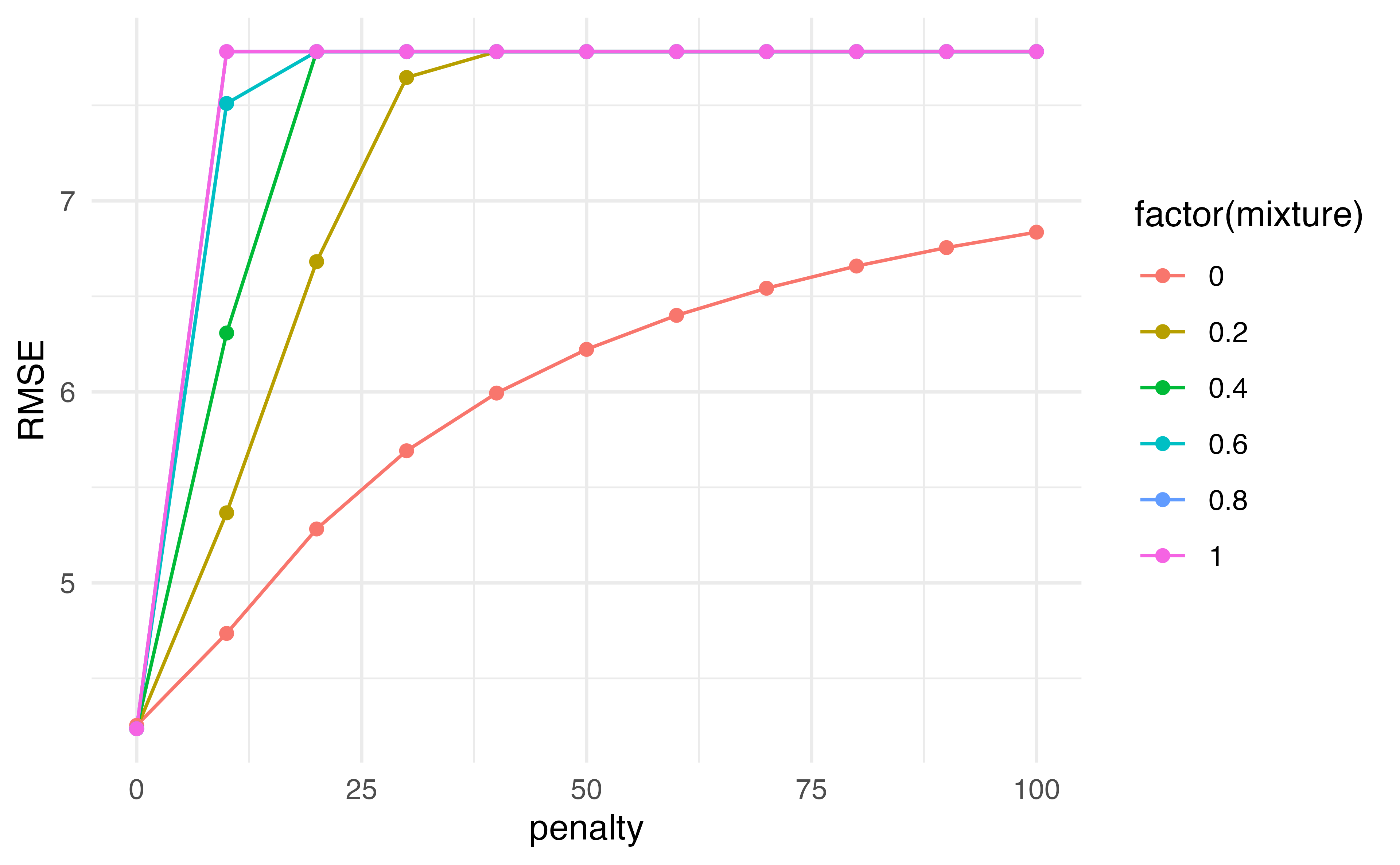

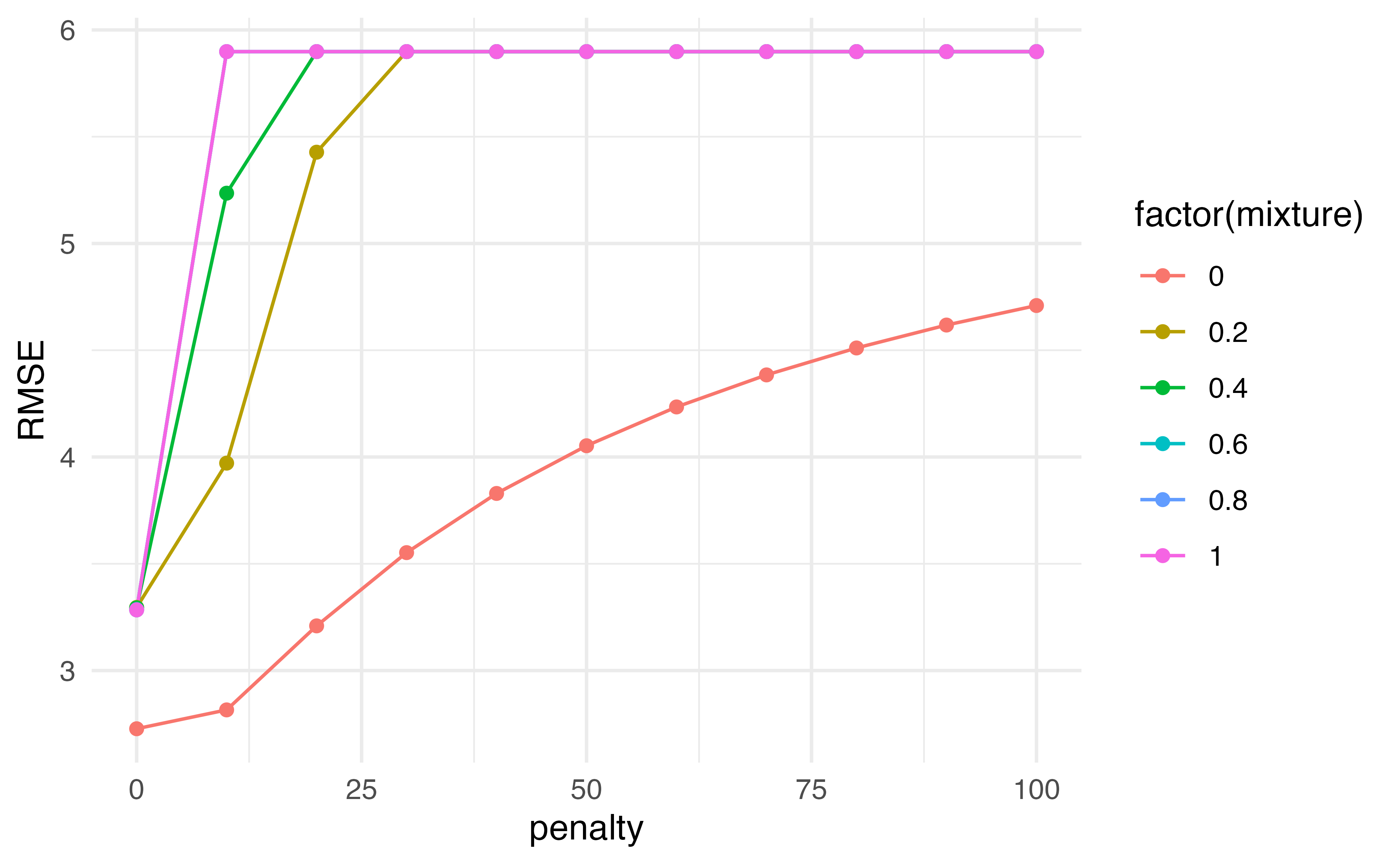
Putting it all together

• Often we can use a combination of all of these tools together
• First split our data
• Do cross validation on just the training data to tune the parameters
• Use last_fit() with the selected parameters, specifying the split data so that it is evaluated on the left out test sample

Putting it all together

auto_split <- initial_split(Auto, prop = 0.5)
auto_train <- training(auto_split)
auto_cv <- vfold_cv(auto_train, v = 5)

rec <- recipe(mpg ~ horsepower + displacement + weight, data = auto_train) |>
  step_scale(all_predictors())

tuning <- tune_grid(penalty_spec,
                     rec,
                     grid = grid,
                     resamples = auto_cv)

tuning |>
  collect_metrics() |>
  filter(.metric == "rmse") |>
  arrange(mean)

# A tibble: 66 × 8
   penalty mixture .metric .estimator  mean     n std_err .config              
     <dbl>   <dbl> <chr>   <chr>      <dbl> <int>   <dbl> <chr>                
 1       0     0.4 rmse    standard    4.03     5   0.197 Preprocessor1_Model23
 2       0     0.2 rmse    standard    4.03     5   0.197 Preprocessor1_Model12
 3       0     0.6 rmse    standard    4.03     5   0.197 Preprocessor1_Model34
 4       0     0.8 rmse    standard    4.04     5   0.198 Preprocessor1_Model45
 5       0     1   rmse    standard    4.04     5   0.198 Preprocessor1_Model56
 6       0     0   rmse    standard    4.05     5   0.196 Preprocessor1_Model01
 7      10     0   rmse    standard    4.60     5   0.206 Preprocessor1_Model02
 8      20     0   rmse    standard    5.16     5   0.217 Preprocessor1_Model03
 9      10     0.2 rmse    standard    5.25     5   0.225 Preprocessor1_Model13
10      30     0   rmse    standard    5.58     5   0.224 Preprocessor1_Model04
# ℹ 56 more rows

Putting it all together

final_spec <- linear_reg(penalty = 0, mixture = 0) |>
  set_engine("glmnet")
fit <- last_fit(final_spec, 
                rec,
                split = auto_split) 
fit |>
  collect_metrics()

# A tibble: 2 × 4
  .metric .estimator .estimate .config             
  <chr>   <chr>          <dbl> <chr>               
1 rmse    standard       4.45  Preprocessor1_Model1
2 rsq     standard       0.691 Preprocessor1_Model1

Extracting coefficients

• We can use workflow() to combine the recipe and the model specification to pass to a fit object.

training_data <- training(auto_split)

workflow() |>
  add_recipe(rec) |>
  add_model(final_spec) |>
  fit(data = training_data) |>
  tidy()

# A tibble: 4 × 3
  term         estimate penalty
  <chr>           <dbl>   <dbl>
1 (Intercept)     42.6        0
2 horsepower      -1.41       0
3 displacement    -1.44       0
4 weight          -3.62       0