Missing Data

Lucy D’Agostino McGowan

The Data

fage : father’s age in years.
mage : mother’s age in years.
mature : maturity status of mother.
weeks : length of pregnancy in weeks.
premie : whether the birth was classified as premature (premie) or full-term.
visits : number of hospital visits during pregnancy.
marital: whether mother is married or not married at time of birth.
gained : weight gained by mother during pregnancy in lbs.
weight : weight of the baby at birth in pounds.
lowbirthweight: whether baby was classified as low birthweight (low) or not (not low).
gender: biological sex of the baby, limited to f or m.
habit : status of the mother as a nonsmoker or a smoker.
whitemom: whether mom identifies as white or not white.

Missing data exploratory analysis

The visdat package is a great way to visualize key information about your dataset
Use the function vis_dat() on your dataframe to see the column types and explore missingness
- This is especially useful for large datasets
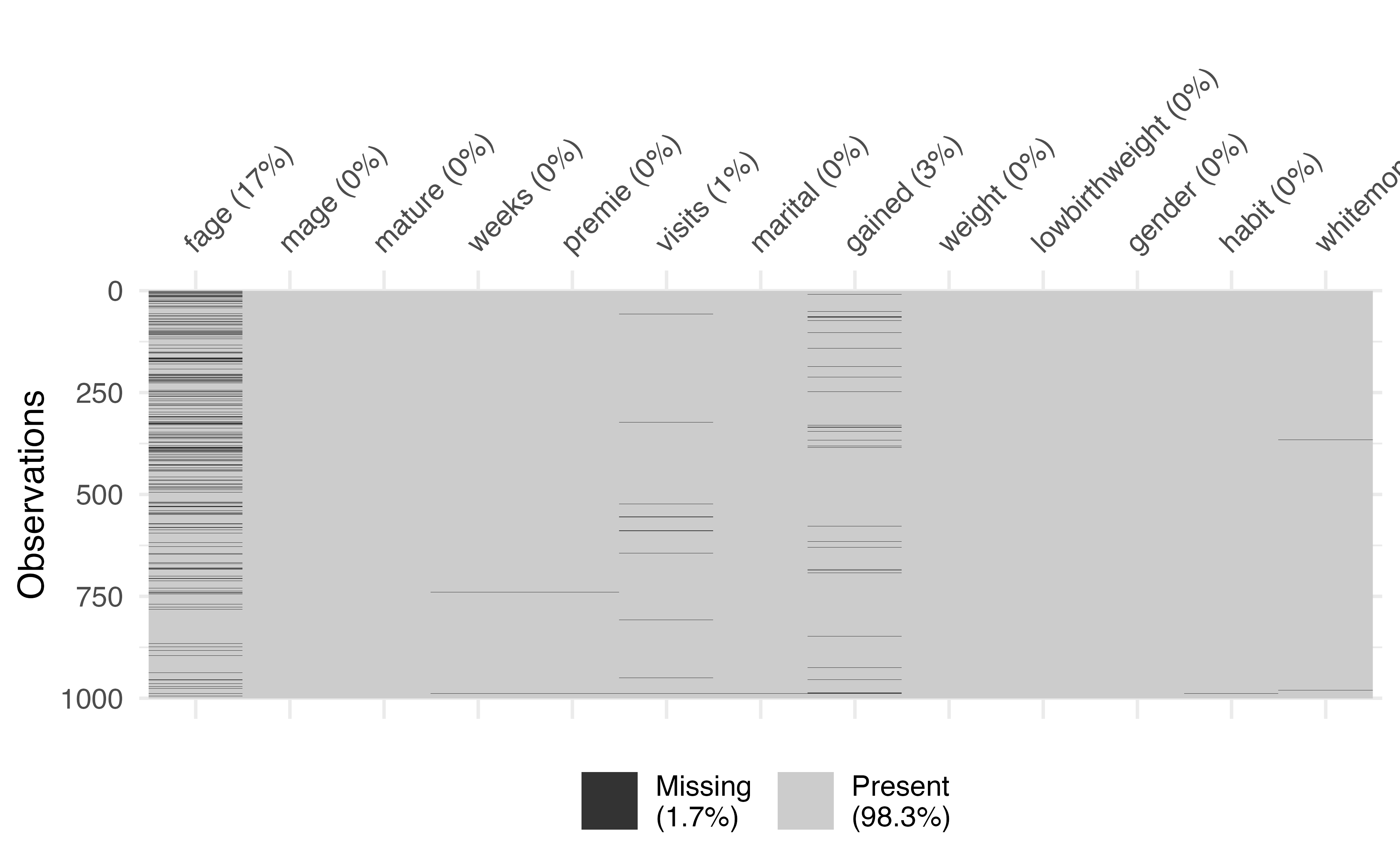
Use the vis_miss() function to learn more about the missing data

`vis_dat()`

library(visdat)
vis_dat(nc)

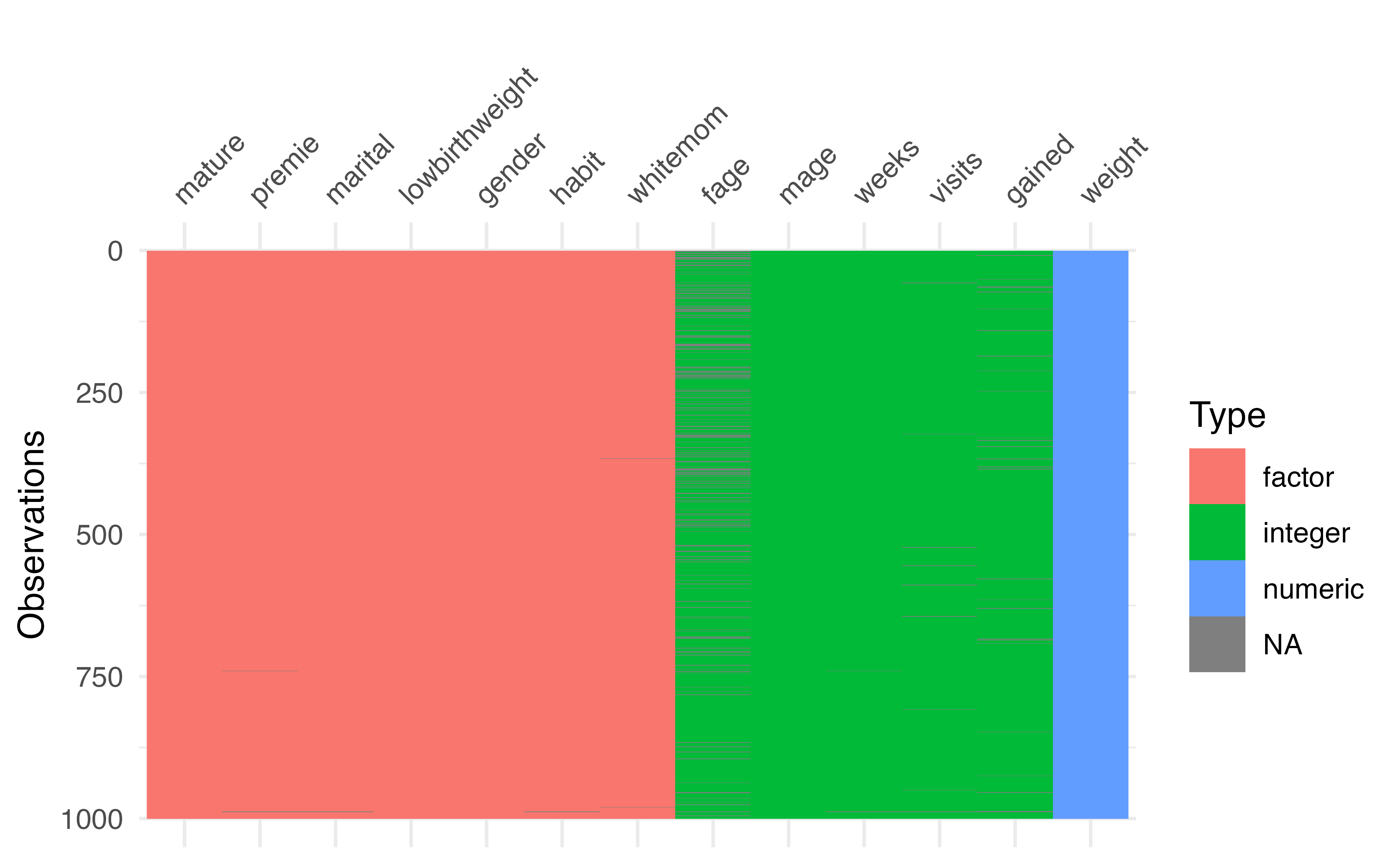
Which column has the most missing data?

`vis_miss()`

vis_miss(nc)

Types of Missingness

Mechanisms of Missingness

There are three classical definitions:

MCAR: Missing Completely at Random
- The probability of being missing is the same for all observations
- Example: Data lost due to random equipment failure

Mechanisms of Missingness

There are three classical definitions:

MAR: Missing at Random
- The probability of being missing depends only on observed data
- Example: Older fathers are less likely to report their age, but conditional on mother’s age, missingness is random

Mechanisms of Missingness

There are three classical definitions:

MNAR: Missing Not at Random
- The probability of being missing depends on unobserved data (the missing values themselves)
- Example: Very young fathers are less likely to report their age because they are young

A More Useful Framework

Rather than MCAR/MAR/MNAR, it’s more practical to think about:

Ignorable missingness: We can safely ignore the missing data mechanism in our analysis
Non-ignorable missingness: We must account for the missing data mechanism

The key question: Is the outcome (Y) or a covariate (X) missing?

When Y is Missing

If your outcome variable is missing:

MAR or MNAR → Non-ignorable
- Complete case analysis can give biased results
- Need careful consideration and possibly imputation
MCAR → Ignorable
- Complete case analysis is unbiased (but inefficient)
- This is a very strong assumption

Bottom line: Missing outcomes are usually problematic and require careful handling

When X is Missing

If your covariate (predictor) is missing:

Pretty much always ignorable!
- Even if MNAR, complete case analysis is typically unbiased
- This might seem surprising, but there’s a good reason…

Visualizing Why Missing X is Ignorable

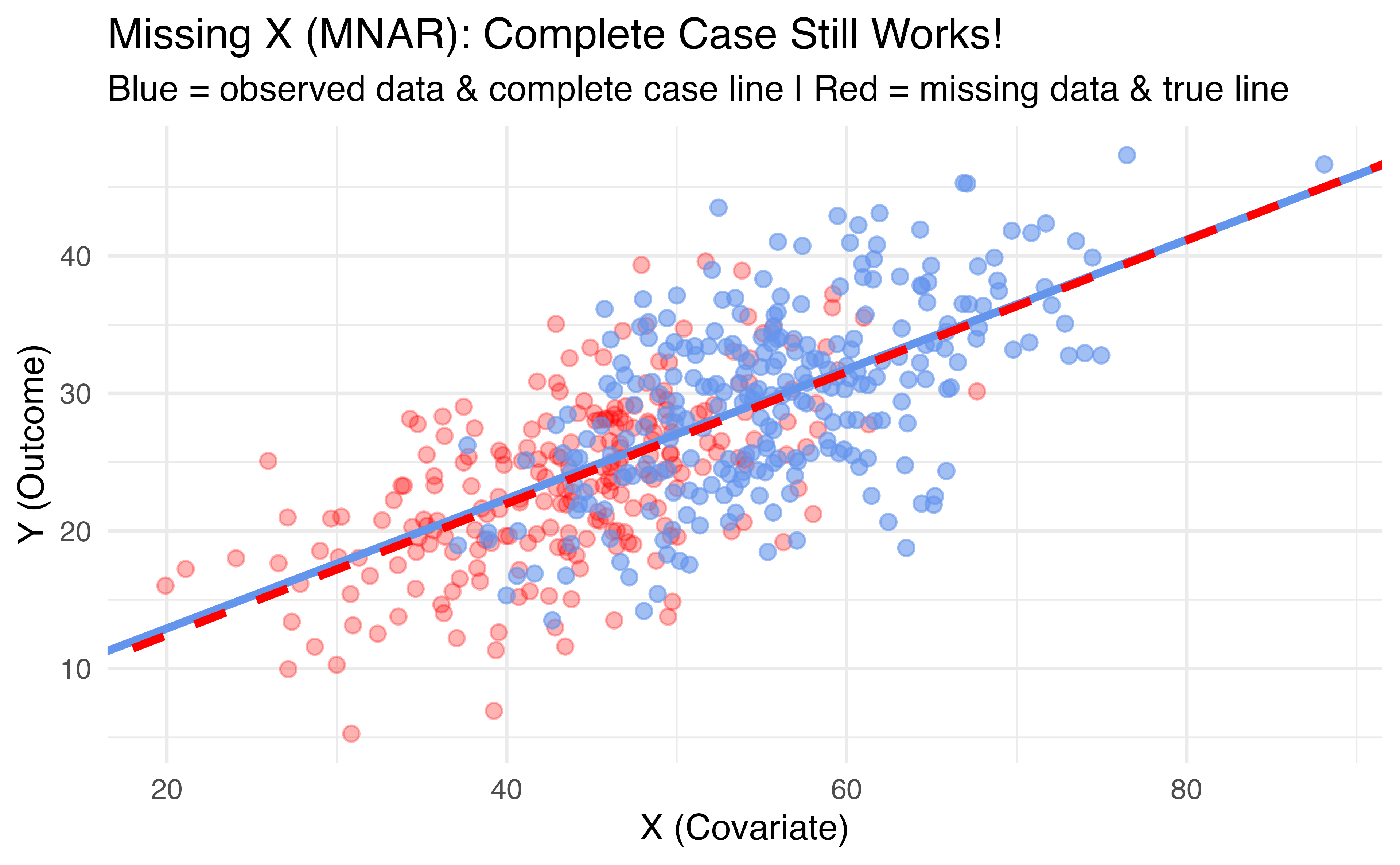
Even though low X values are systematically missing (MNAR), the slope estimate from complete cases (blue) matches the true relationship (red dashed)

What do we do?

There are three typical approaches:

Complete Case Analysis
Available Case Analysis
Imputation

Which to use depends on whether Y or X is missing!

Complete Case Analysis

This is probably what you have done most often
This means we eliminate all rows in the dataset that contain any missing data
The only rows we use are the complete rows, with no missing data

Complete Case Analysis

Advantage: It is easy!

The first step is to create a dataset that only includes rows that are fully observed

nc_complete_case <- nc |>
  drop_na()

## OR
library(tidymodels)
recipe_nc <- recipe(lowbirthweight ~ ., data = nc) |>
  step_naomit(everything()) # this is actual available case behind the scenes

NOTE It is important that you hold on to the original data somewhere when doing complete case analysis, we may need to go back and look at the rows we dropped.

Complete case analysis

When doing complete cases analysis, it is important to always note how many observations are dropped.

n_cc <- nrow(nc_complete_case)
n <- nrow(nc)
n - n_cc

[1] 200

(n - n_cc) / n

[1] 0.2

Here we are dropping 200 rows, losing 20% of the data

When to Use Complete Case Analysis

Use complete case analysis when:

Only covariates (X) are missing
- This is ignorable regardless of mechanism (MCAR/MAR/MNAR)!
- You lose efficiency but not validity

When to Use Complete Case Analysis

Be cautious when:

The outcome (Y) is missing
- Only safe if MCAR (very strong assumption)
- Otherwise likely biased

Disadvantages of Complete Case Analysis

What issues might there be with simply deleting 20% of your sample?

We reduce our sample size (loss of efficiency)
If Y is missing and not MCAR: biased estimates

Disadvantages of Complete Case Analysis

What issues might there be with simply deleting 20% of your sample?

We could lose the representative nature of our data
- What if the data is missing for a reason?
- What if a particular group of people refused to answer a question, so by conducting a complete case analysis we completely remove that group of people from the data set?

Available Case Analysis

Suppose there are 30 variables, but we only need to use 25 in our analysis
Available case analysis means we ignore any missing data in the 5 variables we don’t plan to use and eliminate all rows with missing data in our desired 25 variables

Available Case Analysis

Advantages: Same as complete case analysis (fast and easy!)

Disadvantages: Same as complete case analysis, with one important note:

Safe if only the predictors (X) we’re using are missing
Problematic if the outcome (Y) is missing and not MCAR

Available Case Analysis

nc_available_case <- nc |>
  drop_na(fage, mage, marital, lowbirthweight)

## OR
recipe_nc <- recipe(lowbirthweight ~ mage + fage + marital, data = nc) |>
  step_naomit(all_predictors(), all_outcomes())

n_ac <- nrow(nc_available_case)
n - n_ac

[1] 171

(n - n_ac) / n

[1] 0.171

When to Consider Imputation

Imputation becomes important when:

The outcome (Y) is missing (and not MCAR)
You want to preserve sample size/power
Multiple variables have missingness
You’re doing more complex analyses

For our examples: We’ll focus on imputing missing covariates (X), which is the most common scenario in practice.

Imputation Models Must Be Congenial

Congeniality: A Critical Concept

When imputing missing data, your imputation model must be congenial with your analysis model.

Congeniality means: The imputation model must include at least all the variables in your analysis model (and ideally more!)

Why is this important?

What Happens with Uncongenial Models?

Suppose your analysis model is: \(\text{lowbirthweight} \sim \text{fage} + \text{mage} + \text{habit}\)

But you impute fage using only: \(\text{fage} \sim \text{mage}\)

Problem: You’ve ignored the relationship between fage and habit!

Your imputed values won’t reflect how father’s age relates to smoking habits
This can bias your final analysis results
The more important habit is, the worse the bias

Congenial Imputation: Best Practices

Your imputation model should include:

All variables in your analysis model (predictors)
Additional auxiliary variables that might help predict missingness
Variables related to the missing data mechanism

Why Include the Outcome in Stochastic Imputation?

This might seem counterintuitive, but you should include Y when imputing X if you are using stochastic imputation (like multiple imputation):

The relationship between X and Y should be preserved in imputed values
Leaving out Y can attenuate (weaken) the relationship in your analysis
Not doing so leads to bias (if the imputation model is stochastic)
Most of imputation methods we will see in this class are deterministic, so do not need the outcome

Imputation

To impute all the missing values in this data set, we are going to:

Estimate values for all the missing values in the original data set
Fill in the missing data with these estimates. This is called completing the data
End up with a data set that has the same dimensions as the original nc data set, but with no missing data
Proceed with our modeling

Getting started

There are a lot of techniques we can use for imputation.

The hardest step in this process is deciding which technique might be appropriate
We are going to explore a few commonly used techniques, and discuss the pros and cons of each

`fage`: Father’s Age

Let’s look at one variable with a lot of missing data: fage (a covariate)
There are 171 rows that are missing this variable
For example, here is row 1:

`fage`: Father’s Age

Let’s look at one variable with a lot of missing data: fage (a covariate)
There are 171 rows that are missing this variable
For example, here is row 1:

# A tibble: 1 × 13
   fage  mage mature    weeks premie visits marital gained weight lowbirthweight
  <int> <int> <fct>     <int> <fct>   <int> <fct>    <int>  <dbl> <fct>         
1    NA    13 younger …    39 full …     10 married     38   7.63 not low       
# ℹ 3 more variables: gender <fct>, habit <fct>, whitemom <fct>

We need to decide how to impute (estimate the missing values) for father’s age

Technique 1: Unconditional Mean Imputation

One of the simplest techniques for imputing such values is called unconditional mean imputation, or UMI
This imputation technique involves filling in missing values by looking at all rows that have observed information for the variable of interest, and computing the mean of that variable
We then impute all rows that are missing the variable by plugging in the mean
The idea behind this technique is that if we don’t know what a missing data value should be, it may be reasonable to just plug in the average value

Technique 1: Unconditional Mean Imputation

For our variable of interest, fage, we can conduct unconditional mean imputation (UMI) by:

taking all of the data point for which fage is observed
computing the mean and
replacing all missing fage values with this mean

This will yield a data set that is completed, i.e., has no missing data, in fage

Technique 1: Unconditional Mean Imputation

recipe_nc <- recipe(lowbirthweight ~ ., data = nc) |>
  step_impute_mean(fage)

Technique 1: Unconditional Mean Imputation

Behind the scenes (in practice you don’t need the code below, just showing what the recipe is doing)

nc |>
  summarise(mean_fage = mean(fage, na.rm = TRUE))

# A tibble: 1 × 1
  mean_fage
      <dbl>
1      30.3

nc_mean_impute <- nc |>
  mutate(
    imputed = is.na(fage),
    fage = case_when(
    imputed ~ 30.25573,
    TRUE ~ as.numeric(fage)
  ))

nc_mean_impute %>%
  slice(1)

# A tibble: 1 × 14
   fage  mage mature    weeks premie visits marital gained weight lowbirthweight
  <dbl> <int> <fct>     <int> <fct>   <int> <fct>    <int>  <dbl> <fct>         
1  30.3    13 younger …    39 full …     10 married     38   7.63 not low       
# ℹ 4 more variables: gender <fct>, habit <fct>, whitemom <fct>, imputed <lgl>

Checking our imputations

Once we have completed an imputation process, our next step is ALWAYS to check:

To make sure we actually filled in all the missing values and
To check to see how these imputations compare to the observed data
Did we impute something completely ridiculous, or something that looks reasonable?

Checking our imputations

## Imputed data
nc_mean_imputation <- prep(recipe_nc) |>
  bake(new_data = nc)

nc_mean_imputation |>
  summarise(mean_fage = mean(fage),
            sd_fage = sd(fage))

# A tibble: 1 × 2
  mean_fage sd_fage
      <dbl>   <dbl>
1      30.2    6.16

## Complete case data
nc |>
  drop_na(fage) |>
  summarise(mean_fage = mean(fage),
            sd_fage = sd(fage))

# A tibble: 1 × 2
  mean_fage sd_fage
      <dbl>   <dbl>
1      30.3    6.76

Checking our impuations

Why didn’t the mean change?
How was the standard deviation different?

Considerations: Unconditional Mean Imputation

Our imputed values were all at the mean
This means that we put additional rows exactly 0 standard deviations from the mean
- Standard deviation describes how much we’d expect an average data point to vary from the mean
- Our mean-imputed data set will have a smaller standard deviation than the observed data (more rows are actually exactly at the mean – we did that! so the average distance from the mean is smaller)
- Therefore, unconditional mean imputation generally underestimates the variability in the data

Considerations: Unconditional Mean Imputation

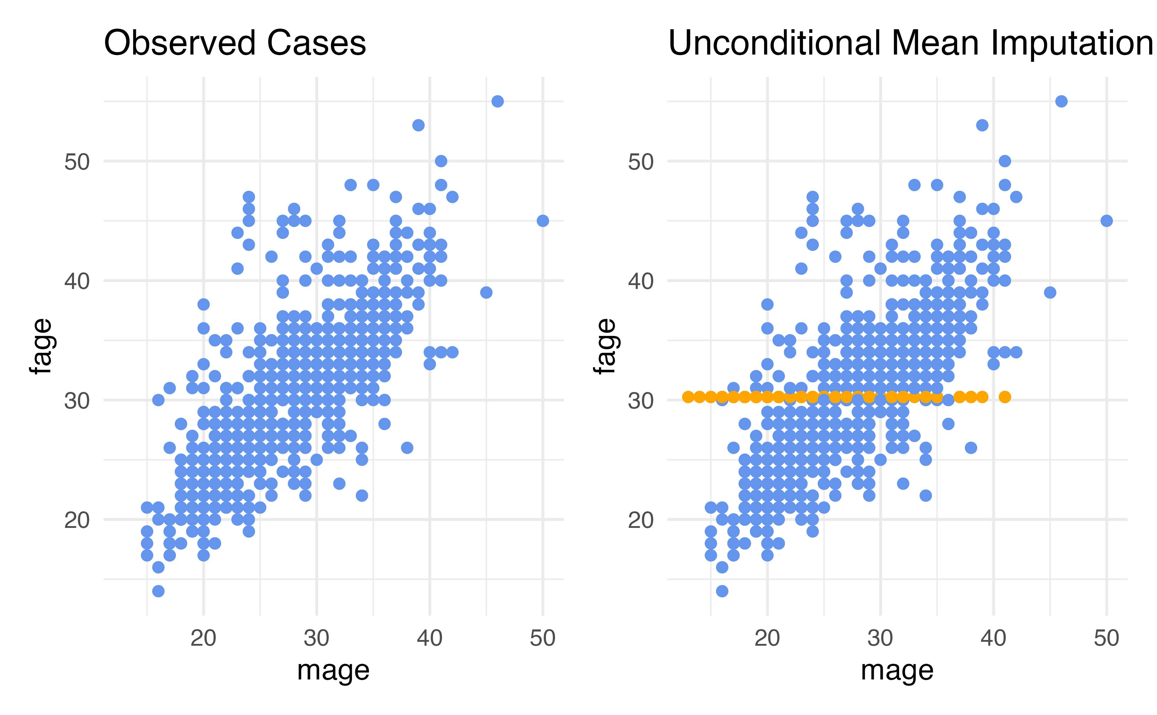
Disadvantages: Unconditional Mean Imputation

Our imputations do not reflect the relationship in the data that exists between fage and mage
This is because we did not include this relationship as part of our imputation strategy!
UMI considers only the marginal distribution of the variable being imputed
It completely ignores the fact that values of fage might be related to another variable present in the data set
As a result, using unconditional mean imputation often results in a distortion of conditional distributions in the data

Considerations for Unconditional Mean Imputation

Pros: It is fast and easy to compute, you can use all observed data
Cons:
- It underestimates the variability in the data
- It often distorts conditional distributions in the data
- It relies on the data being missing completely at random

Conditional Mean Imputation

Rather than computing the marginal mean and putting that in for our missing values, we could calculate a conditional mean, a mean that conditions on our other variables
How do we calculate conditional means?
Linear regression is the simplest way!

Conditional Mean Imputation

recipe_nc <- recipe(lowbirthweight ~ ., data = nc) |>
  step_impute_linear(fage, impute_with = imp_vars(mage))

recipe_nc

Conditional Mean Imputation

Behind the scenes (in practice you don’t need the code below, just showing what the recipe is doing)

nc_cmean_impute <- fit(linear_reg(), 
  fage ~ mage, 
  data = nc) |>
  predict(new_data = nc) |>
  bind_cols(nc) |>
  mutate(
    imputed = is.na(fage),
    fage = case_when(
    imputed ~ .pred,
    TRUE ~ as.numeric(fage)
  ))

nc_cmean_impute

# A tibble: 1,000 × 15
   .pred  fage  mage mature      weeks premie    visits marital gained weight
   <dbl> <dbl> <int> <fct>       <int> <fct>      <int> <fct>    <int>  <dbl>
 1  17.8  17.8    13 younger mom    39 full term     10 married     38   7.63
 2  18.6  18.6    14 younger mom    42 full term     15 married     20   7.88
 3  19.5  19      15 younger mom    37 full term     11 married     38   6.63
 4  19.5  21      15 younger mom    41 full term      6 married     34   8   
 5  19.5  19.5    15 younger mom    39 full term      9 married     27   6.38
 6  19.5  19.5    15 younger mom    38 full term     19 married     22   5.38
 7  19.5  18      15 younger mom    37 full term     12 married     76   8.44
 8  19.5  17      15 younger mom    35 premie         5 married     15   4.69
 9  20.3  20.3    16 younger mom    38 full term      9 married     NA   8.81
10  20.3  20      16 younger mom    37 full term     13 married     52   6.94
# ℹ 990 more rows
# ℹ 5 more variables: lowbirthweight <fct>, gender <fct>, habit <fct>,
#   whitemom <fct>, imputed <lgl>

Conditional Mean Imputation

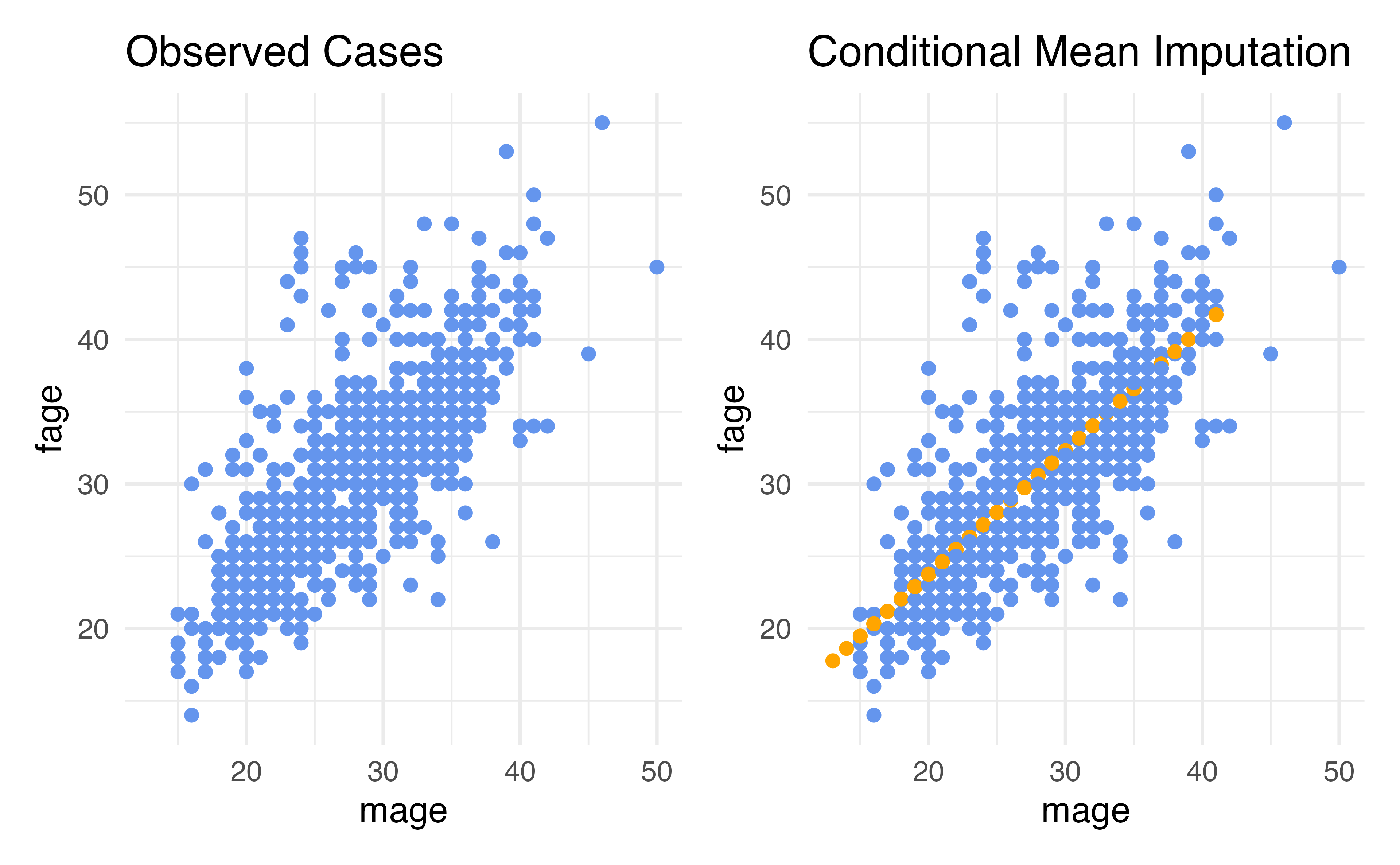
Summary statistics

nc_cmean_imputation <- prep(recipe_nc) |>
  bake(new_data = nc)

nc_cmean_imputation |>
  summarise(mean_fage = mean(fage),
            sd_fage = sd(fage))

# A tibble: 1 × 2
  mean_fage sd_fage
      <dbl>   <dbl>
1      29.7    6.57

nc |>
  drop_na(fage, mage) |>
  summarise(mean_fage = mean(fage),
            sd_fage = sd(fage))

# A tibble: 1 × 2
  mean_fage sd_fage
      <dbl>   <dbl>
1      30.3    6.76

What if we want to include more variables?

What if we think fage is actually conditional on more than just mage?

What if we want to include more variables?

What if we think fage is actually conditional on more than just mage?

recipe_nc <- recipe(lowbirthweight ~ ., data = nc) |>
  step_impute_mode(marital) |>
  step_impute_linear(fage, impute_with = imp_vars(mage, marital))

recipe_nc

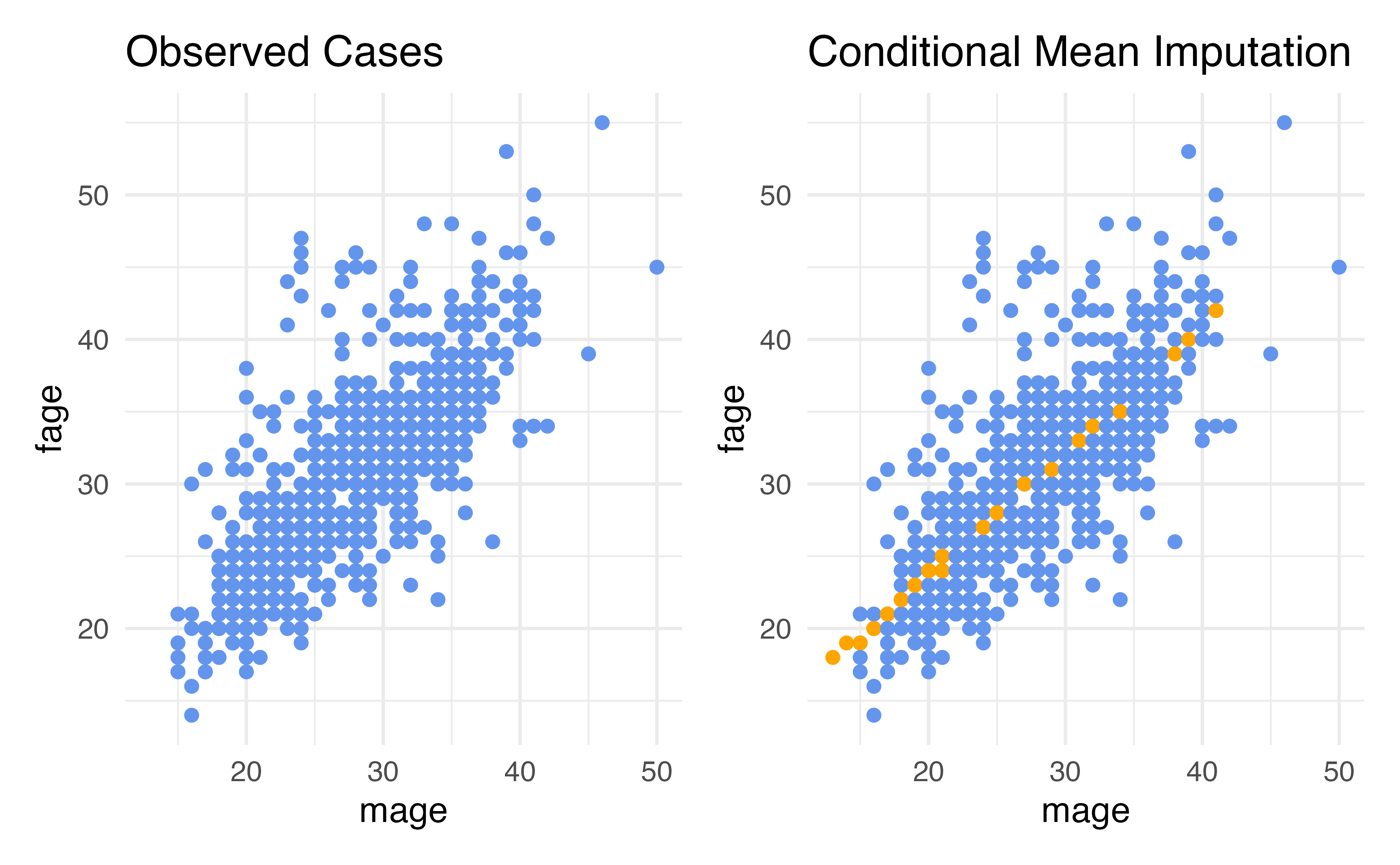
Conditional Mean Imputation

The tidymodels default is to try to impute values using all other predictors
The problem is in order to use this method, the values must not be missing for the other predictors (which is often not the case!)
Let’s see how this errors

Conditional Mean Imputation

recipe_nc <- recipe(lowbirthweight ~ ., data = nc) |>
  step_impute_linear(fage, impute_with = imp_vars(all_predictors()))

wf <- workflow() |>
add_recipe(recipe_nc) |>
  add_model(logistic_reg())

fit(wf, data = nc)

Warning: There were missing values in the predictor(s) used to impute; imputation did
not occur.

Warning: glm.fit: algorithm did not converge

Warning: glm.fit: fitted probabilities numerically 0 or 1 occurred

══ Workflow [trained] ══════════════════════════════════════════════════════════
Preprocessor: Recipe
Model: logistic_reg()

── Preprocessor ────────────────────────────────────────────────────────────────
1 Recipe Step

• step_impute_linear()

── Model ───────────────────────────────────────────────────────────────────────

Call:  stats::glm(formula = ..y ~ ., family = stats::binomial, data = data)

Coefficients:
       (Intercept)                fage                mage   matureyounger mom  
        -1499.5824             -2.1897              5.1293             44.8299  
             weeks        premiepremie              visits  maritalnot married  
            5.4982             15.0877             -2.6857              2.3088  
            gained              weight          gendermale         habitsmoker  
           -0.3773            221.9656             -6.9561            -12.8116  
     whitemomwhite  
          -11.0732  

Degrees of Freedom: 799 Total (i.e. Null);  787 Residual
  (200 observations deleted due to missingness)
Null Deviance:      493.3 
Residual Deviance: 7.287e-07    AIC: 26

Advantages: Conditional Mean (Regression) Imputation

Our data can be conditionally missing at random – this means that the missingness only needs to be random conditional on the variables that we have included in our imputation model
The variability is closer to what it should be compared to just mean imputation

Disadvantages: Regression Imputation

We need to specify the conditional relationships
So far, we’ve only talked about linear regression, meaning this method only works for continuous variables (it turns out you can use logistic for categorical variables, but then you need to specify a separate imputation method for each type of variable, this can be a lot depending on the size of your data!)
The other variables we use for imputation need to not be missing

Conditional Imputation: KNN

We can use another approach that is more flexible and more forgiving to missing data in the other predictors: K-Nearest-Neighbor
The steps:

Using all predictors requested, calculate distances between observations (this uses a method called “Gower’s distance” which can be used for both continuous and categorical data YAY)
Determine “nearest neighbors”, that is other observations that are the closest to you in terms of distance calculated in (1)
The mode of the nearest neighbors will be filled in for categorical variables and the mean will be filled in for continuous

Conditional Imputation: KNN

recipe_nc <- recipe(lowbirthweight ~ ., data = nc) |>
  step_impute_knn(fage, impute_with = imp_vars(all_predictors()))

## these are the same
recipe_nc <- recipe(lowbirthweight ~ ., data = nc) |>
  step_impute_knn(fage)

Conditional Imputation: KNN

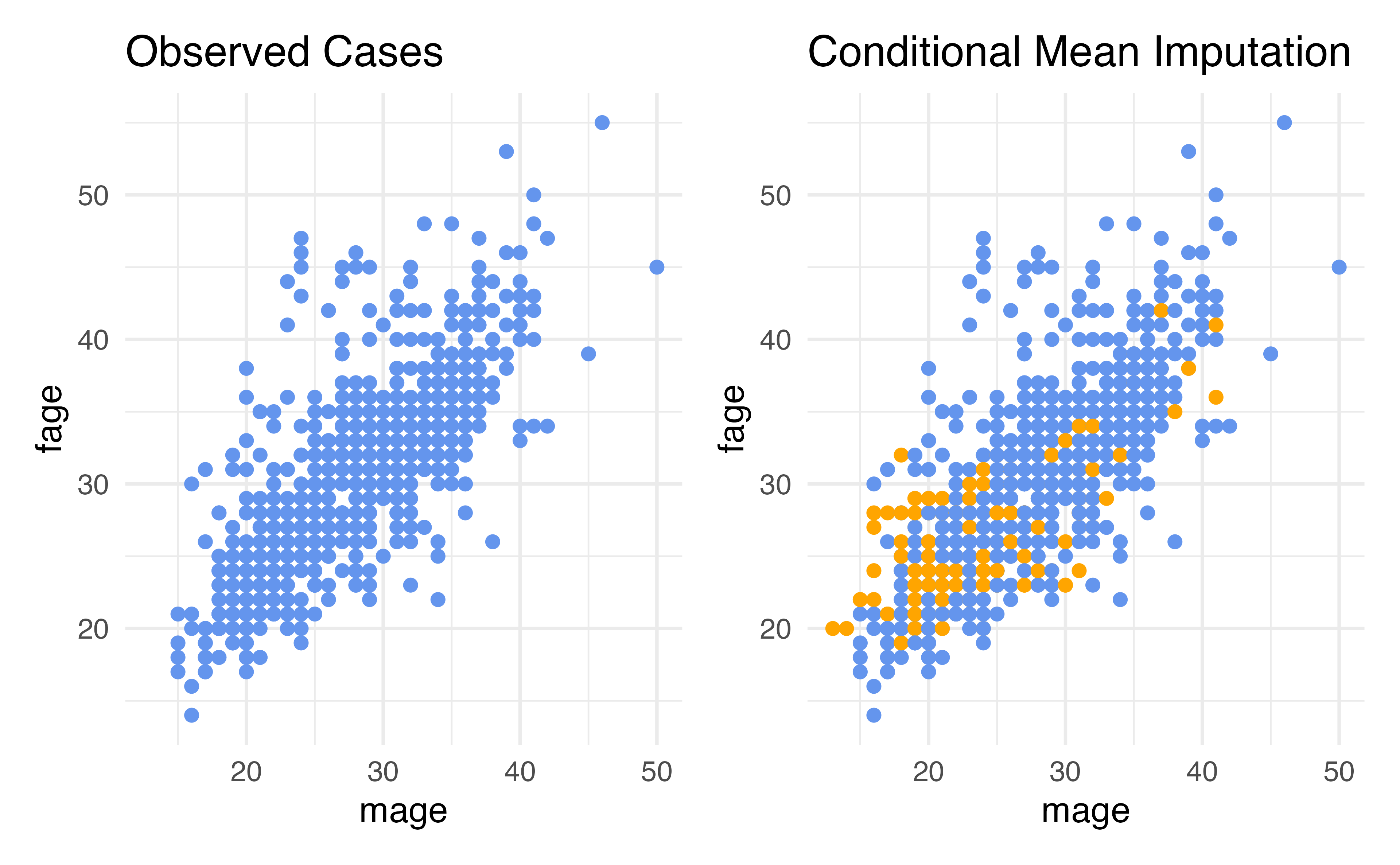
Checking summary statistics

nc_knn_impute <- prep(recipe_nc) |>
  bake(new_data = nc)

nc_knn_impute|>
  summarise(mean_fage = mean(fage),
            sd_fage = sd(fage))

# A tibble: 1 × 2
  mean_fage sd_fage
      <dbl>   <dbl>
1      29.6    6.60

nc |>
  drop_na(fage) |>
  summarise(mean_fage = mean(fage),
            sd_fage = sd(fage))

# A tibble: 1 × 2
  mean_fage sd_fage
      <dbl>   <dbl>
1      30.3    6.76

Advantages: Conditional Imputation: KNN

Our data can be conditionally missing at random – this means that the missingness only needs to be random conditional on the variables that we have included in our imputation model
The variability is closer to what it should be compared to just mean imputation
The method allows for either continuous or categorical variables to be imputed using the same technique
The other variables we are using can be missing as long as they are not mostly missing within each of the K neighbors that end up being chosen (for small percentages of missingness this is reasonable)

Disadvantages: KNN Imputation

We need to specify the conditional relationships (can default to all predictors, though)
Doesn’t account for the full potential variability (we need more advanced techniques like multiple imputation for that)

Summary: Choosing a Method

If only covariates (X) are missing: * Complete/available case analysis is valid (just less efficient) * Imputation can improve efficiency and precision

If the outcome (Y) is missing: * Complete case only valid if MCAR (strong assumption) * Usually need imputation or other careful methods

For imputation: * Unconditional mean: Fast but distorts relationships * Conditional methods (regression, KNN): Better preserve relationships * KNN: Most flexible for mixed data types

Advanced techniques

Chained imputation
Multiple imputation
Multivariate Imputations by Chained Equations (MICE)
- mice package in R is a nice one for this

Missing Data

The Data

Missing data exploratory analysis

vis_dat()

vis_miss()

Types of Missingness

Mechanisms of Missingness

Mechanisms of Missingness

Mechanisms of Missingness

A More Useful Framework

When Y is Missing

When X is Missing

Visualizing Why Missing X is Ignorable

What do we do?

Complete Case Analysis

Complete Case Analysis

Complete Case Analysis

Complete case analysis

When to Use Complete Case Analysis

Use complete case analysis when:

When to Use Complete Case Analysis

Be cautious when:

Disadvantages of Complete Case Analysis

Disadvantages of Complete Case Analysis

Available Case Analysis

Available Case Analysis

Available Case Analysis

Available Case Analysis

When to Consider Imputation

Imputation Models Must Be Congenial

Congeniality: A Critical Concept

What Happens with Uncongenial Models?

Congenial Imputation: Best Practices

Why Include the Outcome in Stochastic Imputation?

Imputation

Imputation

Getting started

fage: Father’s Age

fage: Father’s Age

Technique 1: Unconditional Mean Imputation

Technique 1: Unconditional Mean Imputation

Technique 1: Unconditional Mean Imputation

Technique 1: Unconditional Mean Imputation

Checking our imputations

Checking our imputations

Checking our impuations

Considerations: Unconditional Mean Imputation

Considerations: Unconditional Mean Imputation

Disadvantages: Unconditional Mean Imputation

Considerations for Unconditional Mean Imputation

Conditional Mean Imputation

Conditional Mean Imputation

Conditional Mean Imputation

Conditional Mean Imputation

Conditional Mean Imputation

Summary statistics

What if we want to include more variables?

What if we want to include more variables?

Conditional Mean Imputation

Conditional Mean Imputation

Conditional Mean Imputation

Advantages: Conditional Mean (Regression) Imputation

Disadvantages: Regression Imputation

Conditional Imputation: KNN

Conditional Imputation: KNN

Conditional Imputation: KNN

Checking summary statistics

Advantages: Conditional Imputation: KNN

Disadvantages: KNN Imputation

Summary: Choosing a Method

Advanced techniques

`vis_dat()`

`vis_miss()`

`fage`: Father’s Age

`fage`: Father’s Age